Extracting Gridded Data using RegionGrid
Suppose we have Global Data. However, we are only interested in a specific region (say, the North Central American region as defined in AR6), how do we extract data for this region?
The simple answer is, we use the extractGrid() function, which takes in a RegionGrid and a data array, and returns a new data array for the GeoRegion.
Setup
using GeoRegions
using DelimitedFiles
using CairoMakie

download("https://raw.githubusercontent.com/natgeo-wong/GeoPlottingData/main/coastline_resl.txt","coast.cst")
coast = readdlm("coast.cst",comments=true)
clon  = coast[:,1]
clat  = coast[:,2]
nothing
Let us define the GeoRegion of interest
geo = GeoRegion("AR6_NCA")The Polygonal Region AR6_NCA has the following properties:
Region ID (ID) : AR6_NCA
Parent ID (pID) : GLB
Name (name) : Northern Central America
Bounds (N,S,E,W) : [33.8, 16.0, -90.0, -122.5]
Shape (shape) : Point2{Float64}[[-90.0, 25.0], [-104.5, 16.0], [-122.5, 33.8], [-105.0, 33.8], [-90.0, 25.0]]
(is180,is360) : (true, false)We also define some sample test data in the global domain
lon = collect(0:360); pop!(lon); nlon = length(lon)
lat = collect(-90:90);           nlat = length(lat)
odata = randn((nlon,nlat))
360×181 Matrix{Float64}:
-2.39106 -0.152799 0.667642 … 0.856148 -0.775989 1.51916
-1.28139 1.12587 0.927025 0.459166 0.206874 -1.70895
0.0772726 1.38819 0.782753 -1.25889 0.0696443 0.694788
-1.97782 0.999567 -0.162022 -0.794019 -0.316272 -0.245052
-2.69695 -0.435066 0.015644 1.43762 -0.609822 -0.14286
0.0792229 0.416661 1.15411 … -0.875573 -0.538133 1.94908
0.991503 1.52048 -0.450263 -0.283919 1.70704 0.0203513
-0.119834 0.233131 1.25384 -1.50666 -0.381992 -0.573687
-0.056244 -0.275026 0.115565 -0.0263639 -1.73032 -1.03991
-0.882405 -1.23367 -1.16758 -3.11087 0.441816 -1.35424
⋮ ⋱ ⋮
-2.22929 1.84427 0.0446556 0.879186 1.15951 -0.850466
-0.961954 1.69814 -0.0364694 -1.40959 1.68905 1.28254
-1.20365 -1.18042 -0.244147 1.45581 0.547971 1.85915
-0.683591 1.90203 1.23307 -0.835603 1.16987 1.22902
2.27978 -0.797363 0.167099 … -0.0900065 1.93775 -1.27909
1.01634 -0.538522 -0.332596 1.02968 1.23782 -2.56251
-0.0013758 0.952174 1.01733 0.480017 -1.66254 0.0836861
-0.115814 -0.765204 -0.675883 -0.39169 1.18211 1.47445
0.721631 0.475692 1.39544 -1.10638 0.0525075 -0.322138Our next step is to define the RegionGrid based on the longitude and latitude vectors and their intersection with the GeoRegion
ggrd = RegionGrid(geo,lon,lat)The Polygonal Grid has the following properties:
Grid Bounds (grid) : [124, 107, 271, 239]
Longitude Indices (ilon) : [239, 240, 241, 242, 243, 244, 245, 246, 247, 248 … 262, 263, 264, 265, 266, 267, 268, 269, 270, 271]
Latitude Indices (ilat) : [107, 108, 109, 110, 111, 112, 113, 114, 115, 116, 117, 118, 119, 120, 121, 122, 123, 124]
Longitude Points (lon) : [-122.0, -121.0, -120.0, -119.0, -118.0, -117.0, -116.0, -115.0, -114.0, -113.0 … -99.0, -98.0, -97.0, -96.0, -95.0, -94.0, -93.0, -92.0, -91.0, -90.0]
Latitude Points (lat) : [16.0, 17.0, 18.0, 19.0, 20.0, 21.0, 22.0, 23.0, 24.0, 25.0, 26.0, 27.0, 28.0, 29.0, 30.0, 31.0, 32.0, 33.0]
Region Size (nlon * nlat) : 33 lon points x 18 lat points
Region Mask (sum(mask) / (nlon * nlat)) : 281 / 594Then we extract the data
ndata = extractGrid(odata,ggrd)33×18 Matrix{Float64}:
NaN NaN NaN NaN NaN NaN NaN … NaN NaN
NaN NaN NaN NaN NaN NaN NaN NaN 1.04936
NaN NaN NaN NaN NaN NaN NaN -0.410845 -0.548295
NaN NaN NaN NaN NaN NaN NaN -0.276093 0.0523923
NaN NaN NaN NaN NaN NaN NaN -0.918229 1.16466
NaN NaN NaN NaN NaN NaN NaN … 1.63831 -0.296965
NaN NaN NaN NaN NaN NaN NaN 0.743339 1.99293
NaN NaN NaN NaN NaN NaN NaN -0.916189 -0.0169919
NaN NaN NaN NaN NaN NaN NaN 1.08671 1.10783
NaN NaN NaN NaN NaN NaN NaN 0.223297 1.11682
⋮ ⋮ ⋱
NaN NaN NaN NaN NaN -0.895472 0.360477 NaN NaN
NaN NaN NaN NaN NaN 1.12588 -0.430738 … NaN NaN
NaN NaN NaN NaN NaN NaN 0.13529 NaN NaN
NaN NaN NaN NaN NaN NaN 0.248243 NaN NaN
NaN NaN NaN NaN NaN NaN NaN NaN NaN
NaN NaN NaN NaN NaN NaN NaN NaN NaN
NaN NaN NaN NaN NaN NaN NaN … NaN NaN
NaN NaN NaN NaN NaN NaN NaN NaN NaN
NaN NaN NaN NaN NaN NaN NaN NaN NaNLet us plot the old and new data
fig = Figure()
_,_,slon,slat = coordGeoRegion(geo); slon = slon
aspect = (maximum(slon)-minimum(slon))/(maximum(slat)-minimum(slat))

ax = Axis(
    fig[1,1],width=350,height=350/aspect,
    limits=(minimum(slon)-2+360,maximum(slon)+2+360,minimum(slat)-2,maximum(slat)+2)
)
contourf!(
    ax,lon,lat,odata,
    levels=range(-1,1,length=11),extendlow=:auto,extendhigh=:auto
)
lines!(ax,clon,clat,color=:black)
lines!(ax,slon.+360,slat.+360,color=:red,linewidth=5)

ax = Axis(
    fig[1,2],width=350,height=350/aspect,
    limits=(minimum(slon)-2,maximum(slon)+2,minimum(slat)-2,maximum(slat)+2)
)
contourf!(
    ax,ggrd.lon,ggrd.lat,ndata,
    levels=range(-1,1,length=11),extendlow=:auto,extendhigh=:auto
)
lines!(ax,clon,clat,color=:black)
lines!(ax,slon,slat,color=:red,linewidth=5)

hideydecorations!(ax, ticks = false,grid=false)

resize_to_layout!(fig)
fig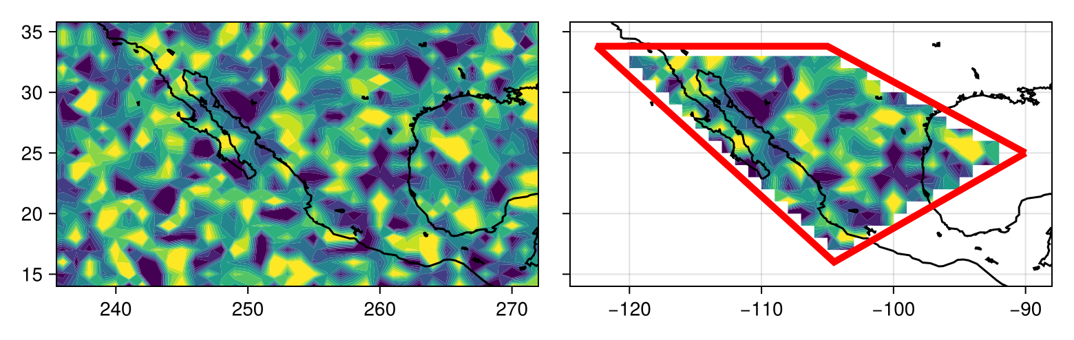
API
extractGrid(
    odata :: AbstractArray{<:Real,N},
    ggrd  :: RegionGrid
) where N <: Int -> Array{<:Real,N}
Extracts data from odata, an Array of dimension N (where N ∈ 2,3,4) that contains data of a Parent GeoRegion, into another Array of dimension N, containing only within a sub GeoRegion we are interested in.
Warning
Please ensure that the 1st dimension is longitude and 2nd dimension is latitude before proceeding. The order of the 3rd and 4th dimensions (when used), however, is not significant.
Arguments
odata: An array of dimension N containing gridded data in the region we are interesting in extracting fromggrd: ARegionGridcontaining detailed information on what to extract
extractGrid!(
    odata :: AbstractArray{<:Real,N},
    ndata :: AbstractArray{<:Real,N},
    ggrd  :: RegionGrid
) where N <: Int -> nothing
Extracts data from odata, an Array of dimension N (where N ∈ 2,3,4) that contains data of a Parent GeoRegion, into ndata, another Array of dimension N, containing only within a sub GeoRegion we are interested in.
This allows for iterable in-place modification to save memory space and reduce allocations if the dimensions are fixed.
Warning
Please ensure that the 1st dimension is longitude and 2nd dimension is latitude before proceeding. The order of the 3rd and 4th dimensions (when used), however, is not significant.
Arguments
odata: An array of dimension N containing gridded data in the region we are interesting in extracting fromndata: An array of dimension N meant as a placeholder for the extracted data to minimize allocationsggrd: ARegionGridcontaining detailed information on what to extract
This page was generated using Literate.jl.