Video Examples
The videos below introduce MeshArrays.jl and present two use cases :
- introduction of
MeshArrays.jlat JuliaCon 2018, for context. - interactive analysis of gridded ocean model output for ECCO.
- simulation of plastic particles following ocean currents.
JuliaCon 2018
MeshArrays.jl was first introduced at JuliaCon in 2018. This video provides some motivation and context for the project.

Interactive Model Analysis
In this demo of interactive visualization of ocean variables, the notebook provides various options for choosing variables and viewing them. Plots etc react to these user selections as illustrated in the video. Code is based on MeshArrays.jl (grids, arrays), OceanStateEstimation.jl (velocity fields, etc), Pluto.jl (notebook), Makie.jl (plotting), and other open source packages.

Another method for interacting with data sets is to use GLMakie.jl or WGLMakie.jl. For example, Tyler.jl can be used to explore high-resolution model output.

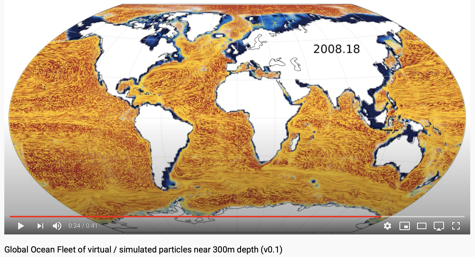
Particle Tracking and Modeling
Here we visualize a simulation of particles moving at a fixed depth in the Ocean (300m depth). This uses Drifters.jl, and MeshArrays.jl underneath, to simulate particle trajectories.
More examples like this, using Julia to run models, and related work in JuliaOcean are available in the longer video below.
