Main Features

• MeshArray, gcmgrid, varmeta
• full Earth grid examples (C-grids)
• vector fields, transports, budgets
• interpolation, distances, collocation
• visualization (via Makie extension)
• particle tracking via IndividualDisplacements.jl

Summary

The MeshArray type is a sub-type of AbstractArray with an outer array where each element is itself a 2D inner array. By default, outer and inner arrays are of all of the standard Array type. However, this setup potentially allows different choices for the outer and inner arrays – for example DistributedArrays and AxisArrays, respectively, could be an option. MeshArrays.jl thus provides a simple but general solution to analyze or e.g. simulate climate system variables. By default the MeshArray type is an alias to the MeshArrays.gcmarray type.

The internals of a MeshArray are regulated by its gcmgrid – a struct containing just a few index ranges, array size specifications, and inter-connection rules. A second lightweight struct, varmeta, contains the MeshArray variable name, its unit, time, and position in grid space. A general approach like this is useful because climate models often involve advanced domain decompositions (see, e.g., Grids), and many variables, which can put a burden on users.

Encoding the grid specification inside the MeshArray data type allows user to manipulate MeshArrays just like they would manipulate Arrays without having to invoke model grid details explicitely. In addition, the provided exchange methods readily transfer data between connected subdomains to extend them at the sides. This makes it easy to compute e.g. partial derivatives and related operators like gradients, curl, or divergences over subdomain edges as often needed for precise computation of transports, budgets, etc using climate model output (see, e.g., Tutorials).

Data Structures

The elements of a MeshArray / are arrays. These elementary arrays typically represent subdomains inter-connected at their edges. The organization and connections between subdomains is determined by a user-specified gcmgrid which is embeded inside each MeshArrays.gcmarray instance.

Interpolate can be used to interpolate a MeshArray to any location (i.e. arbitrary longitude, latitude pair). Exchange methods transfer data between neighboring arrays to extend computational subdomains – this is often needed in analyses of climate or ocean model output.

The current default for MeshArray is the gcmarray type, with various examples provided in the Tutorials.

One of the examples is based on a grid known as LatLonCap where each global map is associated with 5 subdomains of different sizes. The grid has 50 depth levels. Such a MeshArray has a size of (5, 50) (see Tutorials).

The underlying, MeshArray, data structure is:

struct gcmarray{T, N} <: AbstractMeshArray{T, N}
   grid::gcmgrid
   meta::varmeta
   f::Array{Array{T,2},N}
   fSize::Array{NTuple{2, Int}}
   fIndex::Array{Int,1}
   version::String
end

A MeshArray generally behaves just like an Array and the broadcasting of operations has notably been customized so that it reaches elements of each elementary array (i.e. within f[i] for each index of f).

In addition, Mesharray specific functions like exchange can alter the internal structure of a MeshArray by adding rows and columns at the periphery of subdomains.

Embedded Metadata

A MeshArrays.gcmarray includes a gcmgrid specification which can be constructed as outlined below.

struct gcmgrid
  path::String
  class::String
  nFaces::Int
  fSize::Array{NTuple{2, Int},1}
  ioSize::Union{NTuple{2, Int},Array{Int64,2}}
  ioPrec::Type
  read::Function
  write::Function
end

The grid class can be set to LatLonCap, CubeSphere, PeriodicChannel, or PeriodicDomain. For example, A PeriodicChannel (periodic in the x direction) of size 360 by 160, can be defined as follows.

pth=MeshArrays.GRID_LL360
class="PeriodicChannel"
ioSize=(360, 160)
ioPrec=Float32

γ=gcmgrid(pth, class, 1, [ioSize], ioSize, ioPrec, read, write)

Importantly, a gcmgrid does not contain any actual grid data – hence its memory footprint is minimal. Grid variables are instead read to memory only when needed e.g. as shown below. To make this easy, each gcmgrid includes a pair of read / write methods to allow for basic I/O at any time. These methods are typically specified by the user although defaults are provided.

using MeshArrays, Unitful
γ=GridSpec("LatLonCap",MeshArrays.GRID_LLC90)
m=MeshArrays.varmeta(u"m",fill(0.5,2),missing,"Depth","Depth")
D=γ.read(γ.path*"Depth.data",MeshArray(γ,Float64;meta=m))

The above commands define a MeshArray called D which is the one displayed at the top of this section. A definition of the varmeta structure is reported below. The position of a D point within its grid cell is given as x ∈ [0. 1.] in each direction.

struct varmeta
  unit::Union{Unitful.Units,Number,Missing}
  position::Array{Float64,1}
  time::Union{DateTime,Missing,Array{DateTime,1}}
  name::String
  long_name::String
end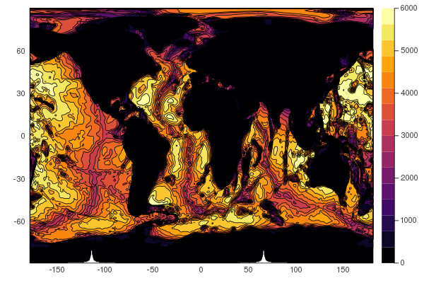

Visualization, Particles, Transports

A simple way to plot a MeshArray consists in using the Makie extension.

By default, for a MeshArray the heatmap command plots each elementary array separately. This is illustrated in Grids and in the Tutorials. If an interpolation scheme is provided then heatmap produces a global map instead. See the geography tutorial for examples. The JuliaClimate Notebooks provide more examples

The vectors tutorial illustrates a common Earth System use case – using gridded flow fields to integrate transports, streamfunctions, budgets, etc. Particle trajectories are readily computed with IndividualDisplacements.jl when velocity fields are provided as MeshArrays.

The MITgcmTools.jl examples shows how MeshArrays.jl can ingest any standard grid from the MIT general circulation model.