Examples
The four examples outlined below form a tutorial of sorts that complements the User Guide. They hopefully provide a useful jumping off point in order to configure IndividualDisplacements.jl for new problems.
Output generated by IndividualDisplacements.jl is in DataFrames.jl tabular format which comes with powerful and convenient analysis methods. They can readily be plotted in space and time using, e.g. , Plots.jl or Makie.jl.
To rerun an example yourself, the recommended method is to copy the corresponding notebook (code) link, paste it into the Pluto.jl prompt, and click open.
Simple Two-Dimensional Flow
notebook (html) ➭ notebook (code)
Simulate an ensemble of displacements (and trajectories) in a simple 2D configuration.
The FlowFields constructor readily wraps a flow field provided in the standard Array format, adds a time range, and returns a FlowFields data structure 𝐹.
All that is left to do at this stage is to define initial positions for the individuals, put them together with 𝐹 into the Individuals data structure 𝐼, and call ∫!(𝐼).
Exercises include the non-periodic domain case, statistics made easy via DataFrames.jl, and replacing the flow field with your own.
Simple Three-Dimensional Flow
notebook (html) ➭ notebook (code)
Set up a three-dimensional flow field u,v,w, initialize a single particle at position 📌, and wrap everything up within an Individuals data structure 𝐼.
𝐼 is displaced by integrating the individual velocity, moving along through space, over time 𝑇. This is the main computation done in this package – interpolating u,v,w to individual positions 𝐼.📌 on the fly, using 𝐼.🚄, and integrating through time, using 𝐼.∫.
The flow field consists of rigid body rotation, plus a convergent term, plus a sinking term in the vertical direction. This flow field generates a downward, converging spiral – a idealized version of a relevant case in the Ocean.
Global Ocean Circulation
notebook (html) ➭ notebook (code)
A simulation of floating particles over the Global Ocean which illustrates (1) using time variable velocity fields, (2) global connections, (3) particle re-seeding, and (4) output statistics.
The flow field is based on a data-constrained ocean model solution. The problem is configured in a way to mimic, albeit very crudely, the near-surface tranport of plastics or planktons.
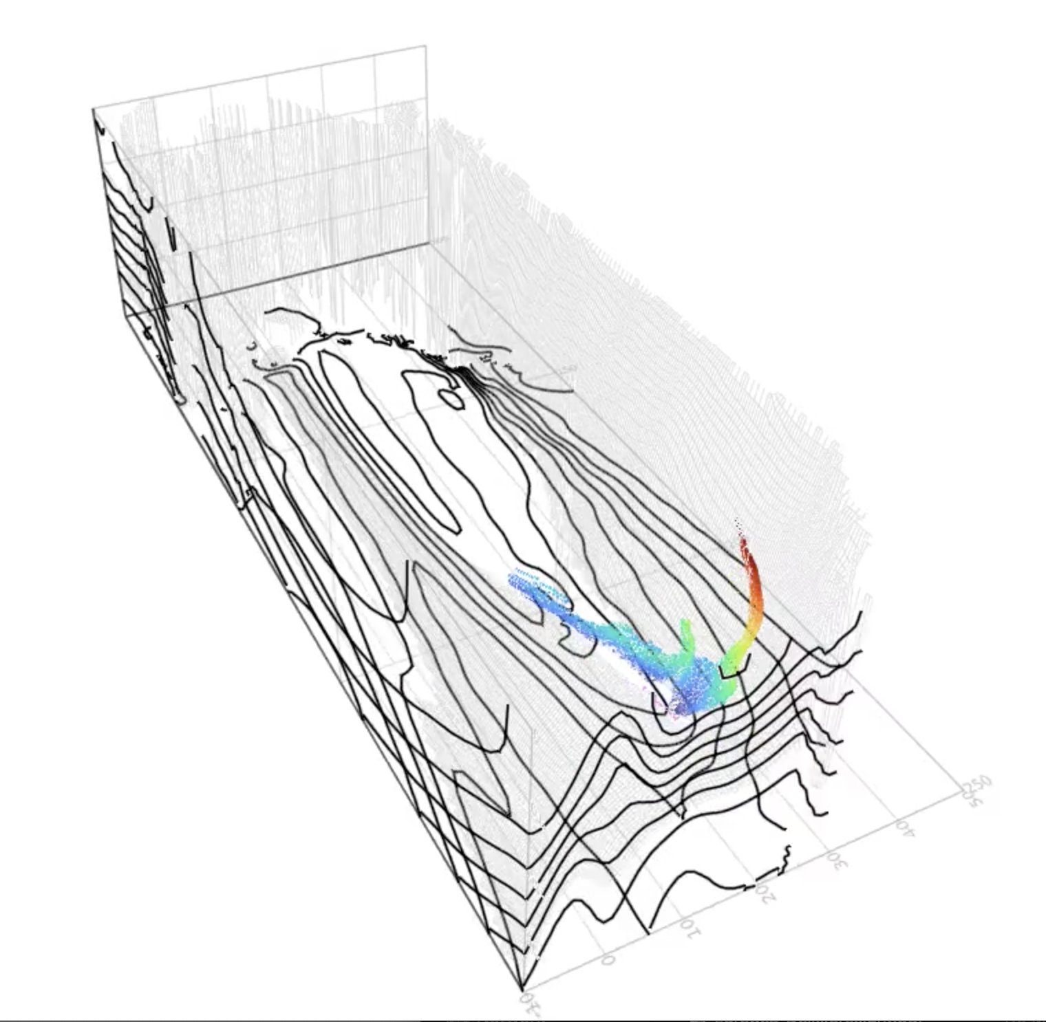
Three Dimensional Pathways
notebook (html) ➭ notebook (code)
A simulation of particles that follow the three-dimensional ocean circulation. This example illustrates (1) the 3D case in a relatistic configuration, (2) tracking the advent or origin of a water patch, and (3) multifacted visualizations in 3D.
The flow field is based on a data-constrained, realistic, ocean model. The problem configuration mimics, albeit very approximately, ocean tracers / coumpounds transported by water masses.
Additional Examples
- Interactivity : notebook (html) ➭ notebook (code)
- Atmosphere : notebook (html) ➭ notebook (code)
- MITgcm : Particle cloud, Detailed look
- Plotting : Plots.jl, Makie.jl, PyPlot.jl
Animations
Below are animations of results generated in Global Ocean Circulation and Three Dimensional Pathways.