User Guide
As shown in the Examples section, the typical worflow is:
- set up a
FlowFieldsdata structure (F) - set up
Individuals(I) with initial position📌andF - displace
Ibysolve!(I,T)followingI.FoverT - post-process by
I.🔧and record information inI.🔴 - go back to
step 2and continue if needed
The data structures for steps 1 and 2 are documented below. Steps 3 and 4 normally take place as part of solve! (i.e. ∫!) which post-processes results, using 🔧, records them in 🔴, and finally updates the positions of individuals in 📌. Since 🔴 is a DataFrame, it is easily manipulated, plotted, or saved in step 4 or after the fact.
using Drifters, CairoMakie
P=Drifters.Gulf_of_Mexico_setup()
F=FlowFields(u=P.u,v=P.v,period=P.T)
I=Individuals(F,P.x0,P.y0);
[solve!(I,P.T .+P.dT*(n-1)) for n in 1:P.nt]
summary(I.🔴)
"481000×4 DataFrame"Plotting functions are provided in the Makie.jl extension, and operated via DriftersDataset.
using MeshArrays, GeoJSON, DataDeps
pol=MeshArrays.Dataset("countries_geojson1")

#prefix="real "; gdf=Drifters.groupby(P.obs,:ID)
prefix="virtual "; gdf=Drifters.groupby(I.🔴,:ID)
options=(plot_type="jcon_drifters",prefix=prefix,xlims=(-98,-78),ylims=(18,31),pol=pol)
LoopC=DriftersDataset(  data=(gdf=gdf,), options=options )
plot(LoopC)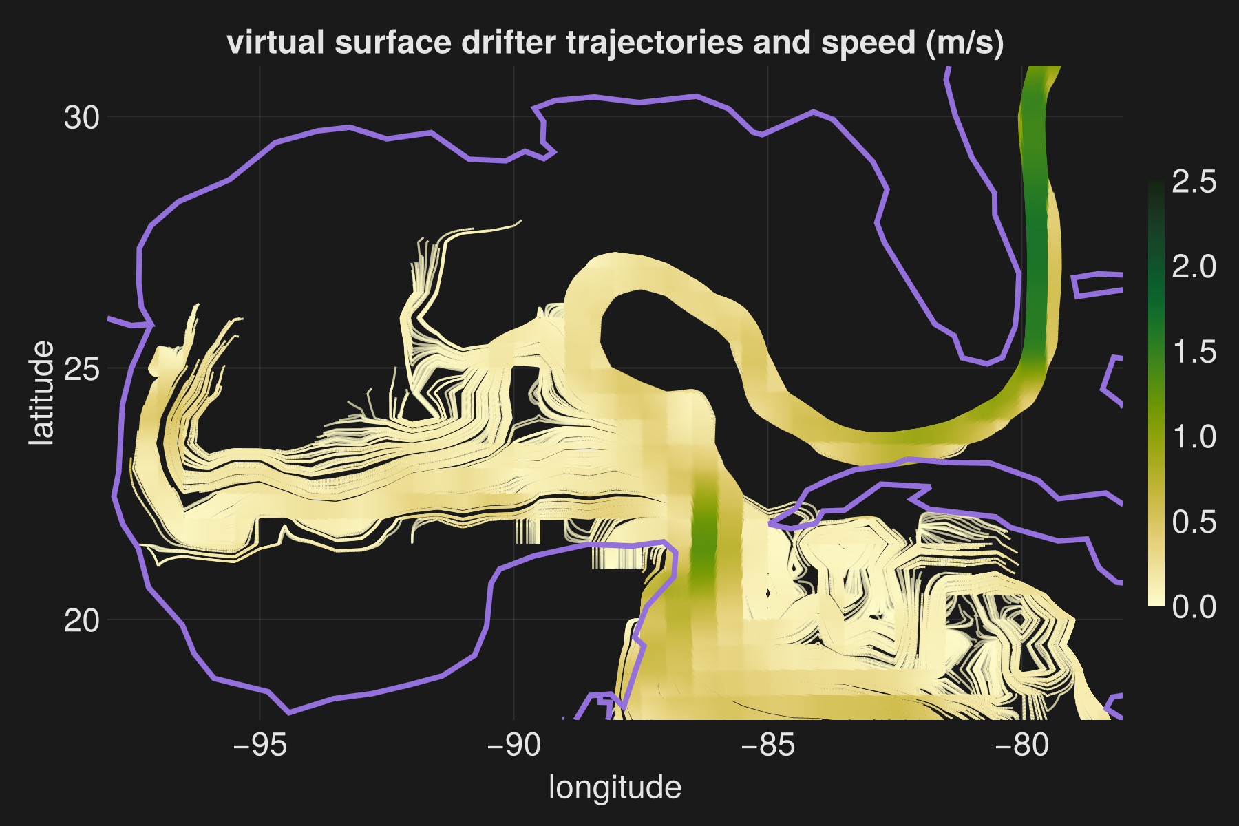
Overview
A central goal of this package is to support scientific analysis of model simulations and observations of materials and particles within the Climate System. The package scope thus includes, for example, drifting plastics in the Ocean or chemical compounds in the Atmosphere.
As a starting point, the package supports all types of gridded model output (on Arakawa C-grids) from the MIT General Circulation Model via the MeshArrays.jl package (docs found here).
By convention, Drifters.jl expects input flow fields to be provided in a uniform fashion (see FlowFields) summarized below:
- normalized to grid index units (i.e. in 1/s rather than m/s units)
- positive towards increasing indices
- using the Arakawa C-grid, with
u(respv) staggered by-0.5point in direction1(resp2) from grid cell centers.
The Examples section documents various, simple methods to prepare and ingest such flow fields (time varying or not; in 2D or 3D) and derive individual displacements / trajectories from them. They cover simple grids often used in process studies, Global Ocean simulations normally done on more complex grids, plotting tools, and data formats.
For an overview of the examples, please refer to the example guide. The rest of this section is focused on the package's data structures and core functions.
Data Structures
The Individuals struct contains a FlowFields struct (incl. e.g. arrays), initial positions for the individuals, and the other elements (e.g. functions) involved in ∫!(I,T) as documented hereafter.
Drifters.AbstractDriftersDataset — Type
abstract type AbstractDriftersDatasetData structure used for plotting. See the docs for examples.
Drifters.FlowFields — Type
abstract type FlowFieldsData structure that provide access to flow fields (gridded as arrays) which will be used to interpolate velocities to individual locations later on (once embedded in an Individuals struct).
Following the C-grid convention also used in MITgcm (https://mitgcm.readthedocs.io) flow fields are expected to be staggered as follows: grid cell i,j has its center located at i-1/2,j-1/2 while the corresponding u[i,j] (resp. `v[i,j]) is located at i-1,j-1/2 (resp. i-1/2,j-1).
By convention :
- time is in seconds but
Tcan also be provided as a vector ofDateTime - position is in grid units. Local coordinates cover
(0 to nx, 0 to ny)if the grid is of size(nx, ny). - velocity fields must be normalized accordingly to grid units (in 1/s rather than m/s) being used in a
FlowFieldsconstructors (whetherArrayorMeshArray)
uvArrays(u0,u1,v0,v1,T)
uvwArrays(u0,u1,v0,v1,w0,w1,T)
uvMeshArrays(u0,u1,v0,v1,T,update_location!)
uvwMeshArrays(u0,u1,v0,v1,w0,w1,T,update_location!)
Using the FlowFields constructor which gets selected by the type of u0 etc.
For exmaple, with Array type in 3D :
F=FlowFields(u,u,v,v,0*w,1*w,[0.0,10.0])Or, with MeshArray` type in 2D :
F=FlowFields(u,u,v,v,[0.0,10.0],func)as shown in the online documentation examples.
Drifters.FlowFields — Method
FlowFields(;    u::Union{Array,Tuple}=[], v::Union{Array,Tuple}=[], w::Union{Array,Tuple}=[],
                period::Union{Array,Tuple}=[])
Simplified FlowFields constructor : using keywords, with time invariant flow fields.
uC, vC, _ = SimpleFlowFields(16)
to_C_grid!(uC,dims=1)
to_C_grid!(uC,dims=2)
F=FlowFields(u=uC,v=vC,period=(0,10.))Drifters.Individuals — Type
struct Individuals{T,N}- Data: 📌 (position), 🔴(record), 🆔 (ID), P (
FlowFields) - Functions: 🚄 (velocity), ∫ (integration), 🔧(postprocessing)
- NamedTuples: D (diagnostics), M (metadata)
The velocity function 🚄 typically computes velocity at individual positions (📌 to start) within the specified space-time domain by interpolating gridded variables (provided via P). Individual trajectories are computed by integrating (∫) interpolated velocities through time. Normally, integration is done by calling ∫! which updates 📌 at the end and records results in 🔴 via 🔧. Ancillary data, for use in 🔧 for example, can be provided in D and metadata stored in M.
Unicode cheatsheet:
- 📌=
\:pushpin:<tab>, 🔴=\:red_circle:<tab>, 🆔=\:id:<tab> - 🚄=
\:bullettrain_side:<tab>, ∫=\int<tab>, 🔧=\:wrench:<tab> - P=
\itP<tab>, D=\itD<tab>, M=\itM<tab>
Simple constructors that use FlowFields to choose adequate defaults:
- Individuals(F::uvArrays,x,y)
- Individuals(F::uvwArrays,x,y,z)
- Individuals(F::uvMeshArrays,x,y,fid)
- Individuals(F::uvwMeshArrays,x,y,z,fid)
Further customization is achievable via keyword constructors:
df=DataFrame( ID=[], x=[], y=[], z=[], t = [])
I=Individuals{Float64,2}(📌=zeros(3,10),🆔=1:10,🔴=deepcopy(df))
I=Individuals(📌=zeros(3,2),🆔=collect(1:2),🔴=deepcopy(df))
Or via the plain text (or no-unicode) constructors:
df=DataFrame( ID=[], x=[], y=[], z=[], t = [])
I=(position=zeros(3,2),ID=1:2,record=deepcopy(df))
I=Individuals(I)Drifters.TimeAxis — Type
struct TimeAxis{Ty} <: AbstractTimeAxisTime axis specification for FlowFields data structure. This un-mutable specification describes the overall range of simulations that can be performed using the FlowFields.
- initial : beginning of simulation period
- final : end of simulation period
- origin : beginning of the valid time period, when flow fields are available
- horizon : end of the valid time period, when flow fields are available
- climatology : false by default ; but can be set to true for time-periodic flow fields.
Rules :
- In most simple cases
origin,horizonis just the same asinitial,final. - By default
initial,finalandorigin,horizonare set to theFlowField'sTimePeriod. - However, any specification where
initial,finalis withinorigin,horizonis correct. - This more general approach makes it easy to split simulations into smaller intervals.
using Drifters, Dates

D0=DateTime(2000,1,1)
D1=DateTime(2000,3,1)
TA=Drifters.TimeAxis(D0,D1)
TA=Drifters.TimeAxis(D0,D1,D0,D1,false)Drifters.TimePeriod — Type
struct TimePeriod{Ty} <: AbstractTimePeriodTime period for next simulation of Individuals displacement specified as a vector [initial,final]. The value field is a mutable vector that can be changed, e.g. within a time loop when carrying out longer simulations.
Rules :
- if
finalprecedesinitialthen the simulation goes backward in time - in most simple cases,
initial,finalare the same inTimePeriodandTimeAxis. - but any
initial,finalwithin the periods defined in 'TimeAxisworks forTimePeriod`.
using Drifters, Dates

D0=DateTime(2000,1,1)
D1=DateTime(2000,3,1)
TP=Drifters.TimePeriod([D0,D1])
TA=Drifters.TimeAxis(TP)Main Functions
∫!(I,T) displaces individuals I continuously over time period T according to velocity function 🚄, temporal integration method ∫, and post-processor 🔧 (all embedded within I).
Drifters.∫! — Function
∫!(I::Individuals,T::Tuple)Displace simulated individuals continuously through space over time period T starting from position 📌.
- This is typically achieved by computing the cumulative integral of velocity experienced by each individual along its trajectory (∫ 🚄 dt).
- The current default is
solve(prob,Tsit5(),reltol=1e-8,abstol=1e-8)but all solver options from the OrdinaryDiffEq.jl package are available. - After this,
∫!is also equipped to postprocess results recorded into 🔴 via the 🔧 workflow, and the last step in∫!consists in updating 📌 to be ready for continuing in a subsequent call to∫!.
∫!(I::Individuals)Call ∫!(I::Individuals,I.P.T)
The velocity interpolation functions (🚄) carry out the central computation of this package – interpolating gridded flow fields to individual positions 📌. It is normally called via ∫! to integrate velocity 🚄 over a chosen time period.
- Velocity interpolation for several array and grid types.
- Preprocessing and postprocessing methods.
- I/O routines to read (write) results from (to) file.
and other functionalities provided in src/compute.jl and src/data_wrangling.jl are further documented in the Tool Box section. Ingestion of trajectory data which have been collected by the Ocean Drifting Buoy Program (movie) is also supported.