Visualization

Maps

Mapping a ClimGrid is done by using the contourf, contour and pcolormesh functions from the package ClimatePlots.

using ClimateTools # to load the netcdf file
using ClimatePlots # which exports the `contourf` function.
C = ClimateTools.load(filenc, "pr", data_units="mm")
contourf(C)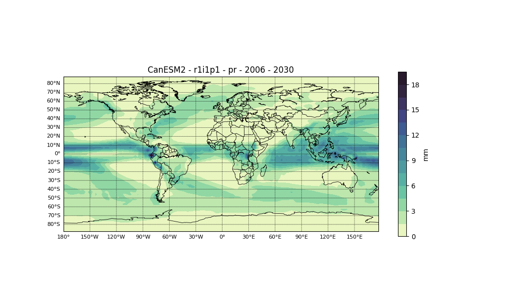

CanESM2

ClimatePlots.contourf — Function

contourf(C::ClimGrid; region::String="auto", level, caxis, titlestr::String, cm::String="", ncolors::Int, center_cs::Bool, filename::String, cs_label::String)

Maps the time-mean average of ClimGrid C. If a filename is provided, the figure is saved in a png format.

Optional keyworkd includes precribed regions (keyword region, see list below). For 4D data, keyword level is used to map a given level (defaults to 1). caxis is used to limit the colorscale. cm is used to manually set the colorscale (see Python documentation for native colorscale keyword), ncolors is used to set the number of color classes (defaults to 12). Set center_cs to true to center the colorscale (useful for divergent results, such as anomalies, positive/negative temprature). cs_label is used for custom colorscale label.

Arguments for keyword region (and shortcuts)

Europe ("EU")
NorthAmerica ("NA")
Canada ("CA")
Quebec, QuebecNSP ("QC", "QCNSP")
Americas ("Ams")
World, WorldAz, WorldEck4 ("W", "Waz", "Weck4")
Greenwich ("Gr")

source

ClimatePlots.contour — Function

contour(C::ClimGrid; region::String="auto", level, caxis, titlestr::String, cm::String="", ncolors::Int, center_cs::Bool, filename::String, cs_label::String)

Maps the time-mean average of ClimGrid C. If a filename is provided, the figure is saved in a png format.

Arguments for keyword region (and shortcuts)

Europe ("EU")
NorthAmerica ("NA")
Canada ("CA")
Quebec, QuebecNSP ("QC", "QCNSP")
Americas ("Ams")
World, WorldAz, WorldEck4 ("W", "Waz", "Weck4")
Greenwich ("Gr")

source

ClimatePlots.pcolormesh — Function

pcolormesh(C::ClimGrid; region::String="auto", level, caxis, titlestr::String, cm::String="", ncolors::Int, center_cs::Bool, filename::String, cs_label::String)

Maps the time-mean average of ClimGrid C. If a filename is provided, the figure is saved in a png format.

Arguments for keyword region (and shortcuts)

Europe ("EU")
NorthAmerica ("NA")
Canada ("CA")
Quebec, QuebecNSP ("QC", "QCNSP")
Americas ("Ams")
World, WorldAz, WorldEck4 ("W", "Waz", "Weck4")
Greenwich ("Gr")

source

Note that the functions plots the climatological mean of the provided ClimGrid. Multiple options are available for region: World, Canada, Quebec, WorldAz, WorldEck4, ..., and the default auto which use the maximum and minimum of the lat-long coordinates inside the ClimGrid structure (see the documentation of contourf for all region options).

Timeseries

Plotting timeseries of a given ClimGrid C is simply done by calling plot. This returns the spatial average throughout the time dimension.

using ClimateTools
using ClimatePlots
poly_reg = [[NaN -65 -80 -80 -65 -65];[NaN 42 42 52 52 42]]
# Extract tasmax variable over specified polygon, between January 1st 1950 and December 31st 2005
C_hist = ClimateTools.load("historical.nc", "tasmax", data_units="Celsius", poly=poly_reg, start_date=Date(1950, 01, 01), end_date=Date(2005, 12, 31)))
# Extract tasmax variable over specified polygon, between January 1st 2006 and December 31st 2090 for emission scenario RCP8.5
C_future85 = ClimateTools.load("futureRCP85.nc", "tasmax", data_units="Celsius", poly=poly_reg, start_date=Date(2006, 01, 01), end_date=Date(2090, 12, 31)))
C = merge(C_hist, C_future)
ind = ClimateTools.annualmax(C) # compute annual maximum
plot(ind)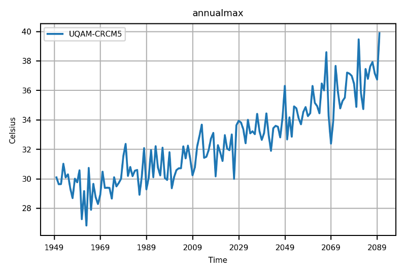

annualmaxtasmax

Note. Time labels ticks should be improved!

The timeserie represent the spatial average of the annual maximum temperature over the following region.

contourf(ind, region = "Quebec")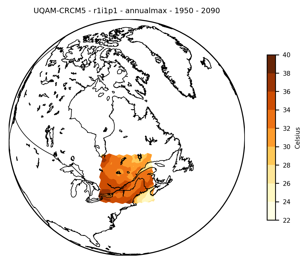

annualmaxtasmax_maps

The map represent the time average over 1950-2090 of the annual maximum temperature.